The MEASUREMENT EQUATION
of a generic radio telescope
AIPS++ Implementation Note nr 185
J.E.Noordam
(jnoordam@nfra.nl)
15 February 1996, version 2.0
File: /aips++/nfra/185.latex
Symbols File:
/aips++/nfra/megi-symbols.tex
Abstract: This note is a step towards an ‘official’ AIPS++ description of the
Measurement Equation, based on an agreed set of names and conventions. The latter
have been defined in a separate TeX file, and can (should) be used in subsequent
AIPS++ documents to ensure consistency.
Contents
1 INTRODUCTION
The matrix-based Measurement Equation (ME) of a Generic Radio Telescope was developed by
Hamaker, Bregman and Sault [2] [3], based on earlier work by Bregman [1]. After discussion by
Noordam [5] and Cornwell [6] [7] [8] [9] [10] [11], the M.E. has been adopted as the generic foundation
of the uv-data calibration and imaging part of AIPS++. In the not too distant future, an ‘official’
AIPS++ description of the ME will be needed, with agreed conventions and nomenclature (see
Appendix A). This note is a step towards that goal.
The heart of the M.E. is formed by the
feed-based ‘Jones’ matrices, which describe the effects of various parts of the observing
instrument on the signal. The main section of this document is devoted to describing the basic
form of the Jones matrices in linear and circular polarisation coordinates. Another section
discusses the conditions under which their order may be modified (matrices do not always
commute).
It is expected that the details of the M.E. (and of this note) will be refined during the first
few iterations of design and implementation of AIPS++. But the structure of the M.E.
formalism as presented here appears to be rich enough to accomodate all existing and
planned radio telescopes. This includes ‘exotic’ ones like cylindrical mirrors, phased arrays,
and interferometer arrays with very dissimilar antennas. Further refinements should only
require the addition of new Jones matrices, or devising new expressions for existing matrix
elements.
In order to test this bold assertion, the various institutes might endeavour to model their own
telescopes in terms of the precise and common language of the M.E., using this note as a reference.
The following ‘rules’ are probably good ones:
- In modelling an instrument, stay as close to the actual physical situation as possible.
Violations of this principle, for whatever reasons, will lead to problems sooner or later.
- It is counterproductive to try and simplify the M.E. to make it ‘look more tractable’. This
practice introduces hidden assumptions, which tend to be forgotten by the programmer,
and unknown to the user.
- Use the suggested nomenclature and conventions.
It is also good to realise that there are two basic forms of ME, which should not be confused: In the
physical form, each instrumental effect is modelled separately by its own matrix. This is useful for
simulation purposes. In the mathematical form, effects are ‘lumped together’ if they cannot be solved
for separately. Example: the various contributions to the receiver gain, and tropospheric
gain.
Acknowledgements: The author has greatly benefited from detailed discussions with
Jayaram Chengalur, Jaap Bregman, Johan Hamaker, Tim Cornwell, Wim Brouw and Mark
Wieringa.
2 THE M.E. FOR A SINGLE POINT SOURCE
For the moment, it will be assumed that there is a single point source at an arbitrary position (direction)
w.r.t.
the fringe-tracking centre, and that observing bandwidth and integration time are negligible. Multiple
and extended sources, and the effects of non-zero bandwidth and integration time will be treated for
the Full Measurement Equation in section 3.
For a given interferometer, the measured visibilities can be written as a 4-element ‘coherency vector’
, which is related to the
so-called ‘Stokes vector’
of the observed source by a matrix equation,
|
| (1) |
The subscripts
and
are the labels of the two feeds that make up the interferometer. The subscripts
and
are the labels of the two output
IF-channels from each feed.
The ‘Stokes matrix’
is a constant
coordinate transformation matrix. It is discussed in detail in section 4 below. The real heart of the M.E. is the ‘direct
matrix product’
of two
feed-based Jones matrices.
The ‘Stokes-to-Stokes’ transmission of a Stokes vector through an ‘optical’ element may be described by
multiplication with a
Mueller matrix
[2] [3]. Using equation 1:
|
| (2) |
Mueller matrices are useful in simulation, when studying the effect of instrumental effects on a test
source .
They can be easily generalised to the full M.E. (see section 3).
2.1 The feed-based instrumental Jones matrices
It will be assumed (for the moment) that all instrumental effects can be factored into feed-based
contributions, i.e. any interferometer-based effects are assumed to be negligible (see section 3). The
interferometer response
matrix then consists of a
‘direct matrix product’
of two
feed-based response matrices, called ‘Jones matrices’. The reader will note that this factoring is the
polarimetric generalisation of the familiar ‘Selfcal assumption’, in which the (scalar) gains are
assumed to be feed-based rather than interferometer-based.
The Jones
matrix for
feed can be decomposed
into a product of several
Jones matrices, each of which models a specific feed-based instrumental effect in the signal
path:
|
| (3) |
in which
| | ionospheric Faraday rotation |
| | atmospheric complex gain |
| | factored Fourier Transform kernel |
| | projected receptor orientation(s) w.r.t. the sky |
| | voltage primary beam |
| | position-independent receptor cross-leakage |
| | commutation of IF-channels |
| | hybrid (conversion to circular polarisation coordinates) |
| | electronic complex gain (feed-based contributions only) |
Matrices between brackets ([ ]) are not present in all systems.
is the
‘Total Voltage Pattern’ of an arbitrary feed, which is usually split up into three sub-matrices:
.
Jones matrices that model ‘image-plane’ effects depend on the source position (direction)
. Some also depend on
the antenna position .
Of course most of them depend on time and frequency as well. The various Jones matrices are treated
in some detail in section 5.
Since the Jones matrices do not always commute with each other, their order is important. In
principle, they should be placed in the ‘physical’ order, i.e. the order in which the signal is affected by
them while traversing the instrument. In practice, this is not always possible or desirable. Section 6
discusses the implications of choosing a different order.
2.2 The Jones matrix of a Tied Array feed
The output signals from the two IF-channels of a ‘tied array’ is the weighted sum of the IF-channel signals
from
individual feeds. A tied array is itself a feed (see definition in appendix A), modelled by its own Jones
matrix. For a single point source, we get:
|
| (4) |
and for an interferometer between two tied arrays
and
with
and
constituent feeds respectively:
|
| (5) |
See also section 6.4. The matrix
models electronic gain effects on the added signal of the tied array
feed .
The
can be solved by the usual Selfcal methods, in contrast to instrumental errors in the constituent
feeds before adding. The latter will often cause decorrellation, and thus closure errors in an
interferometer.
Since a tied array feed can be modelled by a Jones matrix, it can be combined with any other type of
feed to form an interferometer. Examples are the use of WSRT and VLA as tied arrays in
VLBI arrays. Note that this is made possible by factoring the Fourier Transform kernel
into
and
, and
including the latter in the Jones matrices of the individual feeds (see equ 28).
Obviously, the primary beam of a tied array can be rather complicated, but it is fully modelled by equ
4. Moreover, the contributing feeds in a tied array are allowed to be quite dissimilar. It is nor even
necessary for their receptors (dipoles) to be aligned with each other! Thus, equation 4 can also be
used to model ‘difficult’ telescopes like Ooty or MOST, or an element of the future Square
Km Array (SKAI). This puts the crown on the remarkable power of the Measurement
Equation.
2.3 Jones matrices for multiple beams
Using the definition in appendix A, each beam in a multiple beam system should be treated like a
separate logical feed, modelled by its own Jones matrix. Any communality between them can
be modelled in the form of shared parameters in the expressions for the various matrix
elements.
3 THE FULL MEASUREMENT EQUATION
3.1 Summing and averaging
For
‘real’ incoherent sources, observed with a ‘real’ telescope, equ 1 becomes:
|
| (6) |
The visibility vector is integrated
over the extent of the sources (),
over the integration time () and
over the channel bandwidth ().
Integration over the aperture ()
is taken care of by the primary beam properties.
There are only four integration coordinates, whose units are determined by the flux density units in which
is
expressed: .
These coordinates define a 4-dimensional ‘integration cell’. If the variation of
is
linear over this cell, integration is not necessary:
|
| (7) |
in which is the value
for source at the
centre of the cell, for
and . If the
variation of
over the cell can be approximated by a polynomial of order
, then it
is sufficient to calculate only the 2nd derivative(s) at the centre of the cell:
|
| (8) |
Here it is assumed that the 2nd derivatives are be constant over the cell, i.e. the cross-derivatives
are
zero.
3.2 interferometer-based effects
Until now, we have assumed that all instrumental effects could be factored into feed-based
contributions, i.e. we have ignored any interferometer-based effects. This is justified for a
well-designed system, provided that the signal-to-noise ratio is large enough (thermal noise causes
interferometer-based errors, albeit with a an average of zero). However, if systematic errors do occur,
they can be modelled:
|
| (9) |
The diagonal
matrix , the
‘Correlator matrix’, represents interferometer-based corrections that are applied to the uv-data in software
by the on-line system. Examples are the Van Vleck correction. In the newest correlators, it approaches a
constant ().
|
| (10) |
The diagonal
matrix
represents multiplicative interferometer-based effects.
|
| (11) |
The 4-element vector
represents additive interferometer-based effects. Examples are receiver noise, and correlator
offsets.
|
| (12) |
In some cases, interferometer-based effects can be calibrated, e.g. when they appear to be constant in
time. It will be interesting to see how many of them will disappear as a result of better modelling with
the Measurement Equation. In any case, it is desirable that the cause of interferometer-based effects
is properly understood (simulation!).
4 POLARISATION COORDINATES
In the signal domain,
the electric field vector
of the incident plane wave can be represented either in a linear polarisation coordinate frame
or a circular polarisation
coordinate frame .
Jones matrices are linear operators in the chosen frame:
|
| (13) |
For linear polarisation coordinates, equation 1 becomes:
|
| (14) |
and there is a similar expression for circular polarisation coordinates. Thus, as emphasised in [2], the Stokes
vector and the
coherency vector
represent the same physical quantity, but in different abstract coordinate frames. A ‘Stokes matrix’
is a coordinate
transformation matrix in the
coherency domain:
transforms the representation from Stokes coordinates (I,Q,U,V) to linear polarisation coordinates
(). Similarly,
transforms to circular polarisation
coordinates (). Following the
convention of [4], we write:
|
| (15) |
-matrices
are almost unitary, i.e. except for a normalising constant:
.
cannot
be factored into feed-based parts. The two Stokes matrices are related by:
|
| (16) |
with
|
| (18) |
Most Jones matrices will have the same form in both polarisation coordinate frames. But
if a Jones matrix is expressed in terms of parameters that are defined in one of the two
frames, it will have two different but related forms. This is the case for Faraday rotation
, receptor orientation
, and receptor cross-leakage
, in which the orientation w.r.t.
the frame plays a role. The
two forms of a Jones matrix
can be converted into each other by the coordinate transformation matrix
and its
inverse:
|
| (19) |
The conversion may be done by hand, using (the elements
may be
complex):
|
| (20) |
|
| (21) |
Applying these general expressions to rotation
and ellipticity
matrices (see Appendix for their definition), the conversions are:
Usually, all matrices in a ‘Jones chain’ will be defined in the same coordinate frame. An
exception is the case where linear dipole receptors are used in conjunction with a ‘hybrid’
to
create pseudo-circular receptors:
in which
represents an electronic implementation of the coordinate transformation matrix
. All
these expressions are equivalent in the sense that, in conjunction with the indicated Stokes matrix,
they produce a coherency vector in circular polarisation coordinates. The choice of which expression
to use depends on whether one wishes to model the feed explicitly in terms of its physical (dipole)
properties, or whether one wishes to regard is as a ‘black box’ circular feed with unknown internal
structure.
5 GENERIC FORM OF JONES MATRICES
In this section, the ‘generic’ form of various
feed-based instrumental Jones matrices (operators) will be treated in some detail.
It will be noted that for each matrix, the 4 elements have been given an ‘official’ name (e.g.
). The
(possibly naive) idea is that, if the structure of the Measurement Equation is more or less complete,
these ‘standard’ matrix elements could be referred to explicitly by their official names in other
AIPS++ documents (and code), for instance to replace them with specific expressions for particular
telescopes or purposes.
The subscript convention is as follows:
is an element of matrix
for feed ,
which models the ‘coupling factor’ for the signal going from
receptor to
IF-channel .
Where possible, the expressions have been reduced to matrices like the diagonal matrix
(), rotation
matrix ()
etc. These are defined in the Appendix.
5.1 Ionospheric Faraday rotation ()
The matrix
represents (ionospheric) Faraday rotation of the electric vector over an angle
w.r.t. the
celestial -frame.
Since
is defined in one of the polarisation coordinate frames, there will be two different forms for
(see
also section 4). For linear polarisation coordinates:
|
| (25) |
In circular polarisation coordinates, the matrix
is a
diagonal matrix which introduces a phase difference, or rather a delay difference. It expresses the fact
that ionospheric Faraday rotation is caused by a (strongly frequency-dependent) difference in
propagation velocity between right-hand and left-hand circularly polarised signals when travelling
through a charged medium like the ionosphere. In terms of the Faraday rotation angle
(see
above), we get:
|
| (26) |
In principle, the Faraday rotation angle is a function of source direction and feed position:
). However,
Faraday rotation is a large-scale effect, so it will usually have the same value for all sources in the primary
beam: .
For arrays smaller than a few km, the rotation angle will usually also be the same for all feeds:
. These
assumptions reduce the number of independent parameters considerably.
5.2 Atmospheric gain ()
The matrix
represents complex atmospheric gain: refraction, extinction and perhaps non-isoplanaticity. Since
does
not depend on a polarisation coordinate frame, there is only one form:
|
| (27) |
The matrix is diagonal because the atmosphere does is not supposed to cause cross-talk. The
diagonal elements are assumed to be equal, because the atmosphere is not supposed to affect
polarisation.
Atmospheric effects in the ‘pupil-plane’ (i.e. originating directly above the feeds) can be modelled with
a complex gain. It is less clear how to deal with effects that originate higher up in the atmosphere, i.e.
between pupil plane and image plane.
A phase screen over the array can be modelled as
in
which the phase is assumed to be a low-order 2D polynomial as a function of the feed position
:
5.3 Fourier Transform kernel ()
The matrix
represents the Fourier Transform kernel, which can also be seen as a phase weight factor). It is
factored into feed-based parts in order to be able to model a tied array (see section 2.2). Since
does
not depend on the polarisation coordinate frame, there is only one form:
|
| (28) |
in which , which depends on
the projected feed position
and the source direction w.r.t.
the fringe tracking centre ,
and .
If , the
interferometer matrix
is a
diagonal matrix with equal elements. This is equivalent to a multiplicative factor of the familiar form
,
i.e. the Fourier Transform kernel or ‘phase weight’ for the baseline
. For small
fields, ,
so
becomes a 2D FT.
The receptors of a feed are practically always co-located, i.e. they have the same phase-centre:
, so
.
But note that it is possible to model a receptors that are not co-located, i.e.
. It is
not immediately obvious why one would want to do such a thing, but it is good to know that the
formalism allows it.
5.4 Projection matrix ()
if
The ‘Projection matrix’ models the projected orientation of the receptors w.r.t. the electrical
frame
on the sky, as seen from the direction of the source (see also section 5.6 below). Since the orientations
are defined in one of the polarisation coordinate frames, there will be two different forms for
(see
section 4). For linear polarisation coordinates:
|
| (29) |
in which is the projected angle
between the positive -axis and
the orientation of receptor
(see also Appendix ??). There is an implicit assumption here that the feed has perpendicular
receptors and is fully steerable, which is the case for the majority of existing telescopes.
See the next section for the case where the projected orientations are not perpendicular
().
For circular polarisation coordinates:
|
| (30) |
It is sometimes useful to introduce an intermediate coordinate frame, attached to the
feed . In that
case: . The ‘offset’
angle between
receptor and the frame
of feed will be zero in
most cases. The angle
is the parallactic angle, i.e. the angle between two great circles through the source, and through the celestial
North Pole and the local zenith respectively. This parallactic angle is zero for an equatorial feed, and varies
smoothly with
for an alt-az feed:
5.5 Projection matrix ()
if
The M.E. formalism must also be able to deal with more ‘exotic’ antennas like
parabolic cylinders (Arecibo, MOST) or horizontal dipole arrays (SKAI). In those
cases, the projected angles of the two receptors will generally not be equal, i.e.
.
NB: The angle of
receptor is defined
w.r.t. the -axis rather
than the -axis. This
ensures that , so
that matrix reduces
to a simple rotation ,
in the common case described in section 5.4 above.
For linear polarisation coordinates
becomes a ‘pseudo-rotation’ (compare with equ 29 above):
|
| (32) |
For circular polarisation coordinates:
The future large radio telescopes may have feeds in the form of dipole arrays, possibly tilted over an
angle
towards the South w.r.t. the local horizontal plane. In that case, the projected angle
between a North-South (NS)
dipole and the -axis differs from
the projected angle between an
East-West (EW) dipole and the -axis
(I hope this is correct now):
5.6 Voltage primary beam ()
The effects of the primary beam are ignored by [2], which deals implicitly with on-axis sources observed by
feeds with fully steerable parabolic mirrors. The AIPS++ M.E. must of course deal with the general case,
including ‘exotic’ telescopes like Arecibo, MOST and SKAI. To this end, we define a total voltage pattern
matrix ,
which fully describes the conversion of the incident electric field (V/m) into two voltages
(V):
|
| (35) |
NB: Since the Jones matrix
is feed-based, it deals with voltage beams. The power beam for
interferometer
is modelled by .
Note that the formalism deals implicitly with interferometers between feeds with quite dissimilar
primary beams.
In practice, it is often convenient to split the matrix
into a
chain of sub-matrices:
- It is always possible to split off a projection matrix :
See sections 5.4 and 5.5 above.
- It is always possible to split off a position-independent leakage matrix :
See section 5.7 below.
This is most useful in the common case of a fully steerable parabolic antenna. The voltage
patterns of its feed(s) have a fixed shape, which are rotated and translated w.r.t. the sky
when pointing the antenna in different directions. What remains after splitting off
and
is an (approximately)
real and diagonal matrix
which decsribes the position-dependent primary beam attenuation and the position-dependent leakage
(see also equation 38 below):
|
| (36) |
As an example, the diagonal elements of
for an idealised axially symmetric gaussian beam and dipole receptorswould look like:
Note that the two receptor beams are each described in their own coordinate frame
and
projected on the sky (see Appendix A). The projection matrix
only takes care of electrical rotation, but not of the rotation of the voltage beam on the
sky!.
Equation 37 illustrates that the voltage beam of a dipole receptor will be slightly elongated in the direction of the
dipole by a factor ,
even if the mirror is perfectly circular and symmetrical. Obviously, the two asymmetric voltage beams
of a feed will not coincide, because they are oriented differently. The resulting position-dependent
difference is one cause of off-axis instrumental polarisation.
In reality, things will be more complicated, especially for off-axis sources. For instance,
standing waves between the primary mirror and the frontend box, or scattering off
support legs, may cause position-dependent leakage terms. Since these cannot be part of
, they must be modelled as
off-diagonal elements of
itself.
In general,
will be more complicated for antennas with less symmetry. In some exotic cases, it may not be very useful
to split off
or even ,
although it is always allowed. In any case, the M.E. formalism offers a framework for the ful
description of the primary beam of any radio telescope that can be conceived.
5.7 Position-independent receptor cross-leakage
()
The off-diagonal elements
and of
describe ‘leakage’ between receptors, i.e. the extent to which each receptor is sensitive to the radiation
that is supposed to be picked up by the other one.
It is customary to split off the position-independent part
and
of this leakage into
a separate matrix :
Usually, the position-dependent leakage coefficients
and
are
assumed to be zero, but that is not always justified.
If the leakage coefficients are determined empirically by calibration, it is not necessary to
know the details of the leakage mechanism. It is sufficient to solve for the elements of
. In
that case, there is only one form:
|
| (39) |
But in many cases, position-independent leakage can be physically explained by deviations
from the nominal
receptor position angles (see ),
and by deviations from
nominal receptor ‘ellipticities’ .
For linear polarisation coordinates:
The sign
gives the approximation for a well-designed system. Often the two receptors are mounted in a single
unit, so position angle deviations caused by mechanical bending of the feed structure are the same for
both: .
One might also argue that ellipticity should be a reciprocal effect, so that
. This is
roughly consistent with WSRT experience, and these two assumptions are implicit in equ 27 of [3].
However, for high accuracy polarisation measurements, the parameters for each receptor should be at
least partly independent.
For circular polarisation coordinates (see equ 22):
Again, the sign gives
the approximation for
and . See equation 34
for an expression for ()
where . The
expression for ()
with is
similar, but with real coefficients, as expected for circular polarisation coordinates.
5.8 Commutation ()
In some systems, the receptor signals can be switched (commuted) between IF-channels for
calibration.
|
| (42) |
5.9 Hybrid ()
In some cases, circularly polarised receptors consist of linearly polarised dipoles, followed by a
‘hybrid’. The latter is an electronic implementation of the coordinate transformation matrix
from
linear to circular polarisation coordinates:
See equation 18 for the definition of .
If no hybrid is present,
is the unit matrix. Any gain effects in these electronic components are
ignored, or rather they are assumed to be ‘absorbed’ by the gain matrix
.
5.10 Electronic gain ()
The matrix
represents the product of all complex electronic gain effects per output
IF-channel
and . It
models the effects of all feed-based electronics (amplifiers, mixers, LO, cables etc). (The correlator
causes interferometer-based effects, which are discussed in section 3).
|
| (44) |
The
sign indicates that electronic cross-talk is assumed to be absent in well-designed systems, i.e.
. Since this kind of crosstalk
is not necessarily reciprocal, .
In reality,
will be a product of many electronic gain matrices, one for each linear electronic component in the system:
Although a solver will not be able to distinguish these different effects from each other, but it is useful
for simulation of instrumental effects.
5.11 Do we need a configuration matrix ()?
NB: This section is a little polemical, and should disappear when things are more settled.
There has been some debate about the concept of a ‘configuration matrix’
, as proposed
by [2], which models the nominal feed configuration. It represents an idealised coordinate transformation
‘from the frame of the rotating antenna mount to the electronic voltage frame’. It models any rotation
of the receptors w.r.t. ‘the antenna mount’, which must be added to the ‘parallactic’ rotation
of the antenna w.r.t.
the sky. also models the
hybrid if present, but it
ignores the primary beam .
Any deviations from this idealised behaviour are covered by the ‘leakage’ matrix
.
However, the proposed
is most suitable for the special case of fully steerable parabolic antennas. The introduction of an
intermediate antenna coordinate frame seems an unnecessary complication in those cases
where the mirror is not steerable, or is absent entirely (like in a dipole array). Moreover,
violates the rules of modelling by lumping together two effects that have nothing to do with each
other, and do not even occur at the same point in the signal path.
In principle it is a good idea to have one matrix that models the transition
from electric fields (V/m) to electric voltages (V), and this is precisely what
does. This very general matrix can be split up if relevant into sub-matrices like
,
and
. The
matrix
has no part in this, since it represents a rearranging of electronic signals (V), just like
(and will come after
if present!). The
projection matrix
takes care of the entire orientation angle of the receptors w.r.t. the sky, which is the only thing that
really counts.
6 THE ORDER OF JONES MATRICES
The Jones matrices in equation 3 generally do not commute, so their order is important. In principle,
the matrices must be placed in the ‘physical’ order, i.e. the order of the signal propagation path. But
in the equations that are enshrined in existing reduction packages, this is often not the case. This begs
the question why these ‘wrong’ equations seem to produce so many good (even spectacular) results.
The question is especially important since a different order often results in considerable gains in
computational efficiency.
The answer is that, for existing (arrays of) circularly symmetric parabolic feeds, many Jones
matrices can be approximated by matrices that do commute with at least some of the
others.
6.1 Overview of commutation properties
We will analyse this in terms of those special matrices (see Appendix for their definition), whose
commutation properties are:
- Unit matrices
commute with all matrices.
- Multiplication matrices ,
i.e. diagonal matrices with equal elements ,
are equivalent to a multiplicative factor. Therefore, they commute with all matrices.
- Diagonal matrices
with unequal elements
commute with each other.
- Pure rotation matrices
commute with each other.
- Pseudo rotation matrices
do not commute wit each other or with pure rotation matrices .
Moreover, there should only be one pseudo rotation matrix in the chain, and it should be to
the left of (i.e. after) all other rotation matrices: .
- Ellipticity matrices
do not commute with each other , except when .
Moreover: .
In order to study the general implications of changing the order of multiplication, we take the two
products
and of
two general matrices (whose elements may be complex):
The difference (i.e. commutation error) between the two matrix products can be expressed as a matrix
:
|
| (46) |
Thus, by taking the wrong matrix order, one makes the following fractional errors of the following
order in the result:
- in the diagonal elements: of the order of ,
i.e. the ratio of non-diagonal and diagonal elements of the original matrices (which is often small).
- in the off-diagonal elements: in the order of ,
i.e. they will be smaller as the diagonal elements of the original matrices are more equal.
If one of the two matrices is diagonal, e.g.
then this reduces to:
|
| (47) |
The (not very surprising) conclusion is that the error caused by taking the wrong matrix order is
smaller when one of the matrices is diagonal, and the values of its diagonal elements are almsot
equal.
6.2 Overview of Jones matrix forms
It is sufficient to discuss the commutation properties of the feed-based Jones matrices because, if
commutes
with and
with
, then
commutes
with :
|
| (48) |
Inspecting the various Jones matrices separately:
| | = pure rotation |
| | = diagonal matrix |
| | = multiplication |
| | = multiplication if (virtually always the case) |
| | = pure rotation if |
| | = diagonal matrix if |
| | = pseudo-rotation if |
| | = A general matrix if |
| | = diagonal matrix if no cross-leakage () |
| | = multiplication if also for all |
| | unit matrix if small leakage, i.e. () |
| | = |
| | if and |
| | = () () |
| | if and |
| | = anti-diagonal matrix: a problem, if present.... |
| | = effectively hidden if present, see equation 24 |
| | = diagonal matrix if no cross-talk |
Problems are caused predominantly by matrices with non-zero off-diagonal elements like
,
, and
if
. Of these, only
is present in all telescopes.
will be a problem
for SKAI, bacause .
6.3 Allowable changes of order
The following changes in the order of Jones matrices is allowed, but only under the indicated
conditions. NB: Some Jones matrices will commute if it can be assumed that the observed source
is compact, dominating, unpolarised and near the centre of the field. This is often the
case.
- If the Faraday angle does not vary over the primary beam,
might be applied in the uv-plane.
will in general commute with
except when
is a pseudo-rotation ().
is diagonal, and will commute with
if it is diagonal. But
will only commute with
if the latter is a multiplication. If there is appreciable cross-leakage,
should stay to the right of ,
which means that in that case
cannot be lumped with
as is often done.
-
is a multiplication, which commutes with everything. If it does not vary over the primary
beam, it can be lumped with .
- If the two receptors of a feed are located at the same position (which is virtually always
the case), the FT kernel matrix
reduces to a multiplication .
This means that the FT can be performed at any desired place in the chain, even to the
right of the Stokes matrix. NB: If ,
it would not be trivial to figure out what the correct position of
should be.
- If the map centre
is different from the fringe tracking centre ,
the FT kernel may be split into a product: .
Since
does not depend on source position,
may be moved to the leftmost part of the chain, i.e. to the uv-plane part.
- If ,
i.e. if all voltage patterns are identical, then
commutes with the Stokes matrix
and may be applied directly to the Stokes vector
in the image plane. This condition is more likely to occur near the beam centre. NB:
Because
does definitely not commute with
if ,
the justification for the practice of applying off-axis instrumental polarisation to
seems a little doubtful.
-
may be moved to the left of
if they are both diagonal matrices, or if
is a multiplication. Since
is diagonal and
is not (except for equatorial mounts), this appears to be an argument in favour of the use of
circular polarisation coordinates. If
is diagonal and almost a multiplication (i.e. ),
may be moved to the left of
at the cost of a small error of the order
(see equation 47).
- If
and
do not commute at all, one can still move
to the left of
by using
Since this re-introduces time-dependent off-diagonal elements into ,
it is not clear how useful this is.
6.4 VisJones and SkyJones
The Jones matrices may split up in two groups:
. In
these terms, the full M.E. (ignoring normalisation factors, see equ 6) becomes:
|
| (49) |
We now see the reason for placing the integration over
and
to the left of
the sum over
sources. Since it is computationally advantageous to minimise the number of Jones matrices that
operate in the image plane, it must be investigated whether Jones matrices that do not depend
on the source position can be moved to the left in the chain, using the rules in section
6.3 above. Depending on the chosen coordinate system, (and always keeping in mind the
conditions for re-ordering Jones matrices), the following split appears to be the maximum
obtainable:
This is what is done implicitly in some existing reduction packages.
6.4.1 Tied Array
For a tied array (ignoring integration and weight factors for the moment), equation 5
becomes:
|
| (53) |
Under extremely favourable conditions, i.e. if:
- individual feed beams per tied array are identical.
- Faraday rotation is the same for an entire tied array
- All receptors of a tied array have the same orientation.
- receptor cross-leakages are small.
- tied array feed signals are corrected before adding.
- there are no delay errors.
then equation 53 can be reduced to:
|
| (54) |
References
[1] J.D.Bregman, J.E.Noordam Matrix formalism for Interferometric
Polarisation Calibration. Internal proposal to AIPS++ project, April 1993.
[2] J.P.Hamaker, J.D.Bregman, R.J. Sault Understanding
Radio Polarimetry I: Mathematical foundations. Accepted by
Astronomy and Astrophysics, Sept 1995. (For a preprint, see
http:://www.nfra.nl/hamaker).
[3] R.J.Sault, J.P.Hamaker, J.D.Bregman Understanding Radio
Polarimetry II: Instrumental calibration of an interferometer array. Accepted
by Astronomy and Astrophysics, Sept 1995. (For a preprint, see
http:://www.nfra.nl/hamaker).
[4] J.P.Hamaker, J.D.Bregman Understanding Radio Polarimetry III:
Interpreting the IAU/IEEE definitions of the Stokes parameters Submitted
to Astronomy and Astrophysics, Oct 1995. (For a preprint, see
http:://www.nfra.nl/hamaker).
[5] J.E.Noordam Some practical aspects of the matrix-based Measurement
Equation of a generic radio telescope. AIPS++ Implementation note 182
(June 1995)
[6] T.J.Cornwell Calibration and Imaging using the Measurement Equation for
the Generic Interferometer. AIPS++ Implementation note 183 (July 1995)
[7] T.J.Cornwell The Generic Interferometer I: Overview of Calibration and
Imaging AIPS++ Implementation note 183 (August 1995)
[8] T.J.Cornwell The Generic Interferometer II: Image Solvers AIPS++
Implementation note ... (revised version, Aug 1995) developing
[9] T.J.Cornwell The Generic Interferometer III: Analysis of Calibration and
Imaging AIPS++ Implementation note ... (Nov 1995) developing
[10] T.J.Cornwell, M.H.Wieringa The Generic Interferometer IV: Design of
Calibration and Imaging AIPS++ Implementation note ... (Dec 1995)
developing
[11] T.J.Cornwell The Generic Interferometer V: Specification of Calibration and
Imaging AIPS++ Implementation note ... (Sept 1995) developing
[12] A.R.Thompson, J.M.Moran,
G.W.Swenson Interferometry and Synthesis in Radio Astronomy. John Wiley
and Sons (1986)
[13] R.A.Perley, F.R.Schwab, A.H.Bridle Synthesis Imaging in Radio
Astronomy. Astronomical Society of the Pacific Conference Series, Vol 6
(1989)
A APPENDIX: CONVENTIONS
A consistent nomenclature and precise definitions are extremely important for a software package like
AIPS++, which aspires to be a ‘world reduction package’, and to which workers with a large
spacetime separation are supposed to contribute. One of the most sensitive areas in this respect
is the Measurement Equation, which underlies the central subject of uv-calibration and
imaging.
However, it is not easy to define, adopt and enforce the use of a suitable set of conventions. This
appendix is a hopefully useful step in that process. It proposes coordinate conventions and some
definitions (notably the one for feed!), and lists symbols that have been defined in a separate TeX file
(referred to as \include(megi-symbols) in this LaTeX document). The TeX syntax is shown in small
print (e.g. \FeedI), for easy reference.
A.1 Some definitions
The following definitions are displayed in a distinctive font throughout the text of this document in
order to emphasize that they have been defined explicitly.
- A receptor (\Receptor) converts the incident electric field into a voltage.
- An IF-channel (\IFchannel) is one of the two output signals of a feed, one for each
‘polarisation’. NB: The signals in a pair of IF-channels may be a linear combination of
the signals of the two receptors.
- A feed (\Feed) is the most fundamental concept of the M.E. formalism, since
Jones-matrices are feed-based. Although a feed may sometimes have only one receptor, it
usually has two, which is necessary and sufficient to fully sample the incident e.m. field.
Each feed is modelled by its own Jones matrix. NB: A feed is a logical concept. Thus,
the same physical feed may be involved in several logical feeds, e.g. for different beams in
a multi-beam instrument, or for different spectral windows.
- An antenna (\Antenna) is a physical grouping of feeds. NB: As a concept, it tends to play
a rather confusing role in the M.E. discussions.
- An interferometer (\Interferometer) is the combination of two feeds. Its output is
a visibility of 1-4 spectra, depending on the number of IF-channels per feed. NB:
Sometimes the combination of two individual IF-channels is also called an interferometer.
In that case, its output is a single spectrum.
- A telescope (\Telescope) is an entire instrument. It can be a single dish (e.g. GBT) or
an aperture synthesis array (e.g. ATCA).
- A projected (\Projected) angle is an angle projected on the plane perpendicular to the
propagation direction (the -axis).
A.2 Labels, sub- and super-scripts
| | \FeedI,\FeedJ | feed labels |
| | \RcpA,\RcpB | receptor labels, two per feed. |
| | \IFP,\IFQ | IF-channel labels,two per feed. |
| | \RPol,\LPol | circular polarisation (right, left) |
| | \XPol,\YPol | linear polarisation (N-S, E-W) |
| | A\ssLin,A\ssCir | superscripts for linear and circular polarisation |
| | A\ssI,A\ssIJ | feed subscripts |
The subscript convention of matrix elements is as follows:
refers to a matrix
element of matrix for
feed , which models the coupling
of the signal going from receptor
to IF-channel .
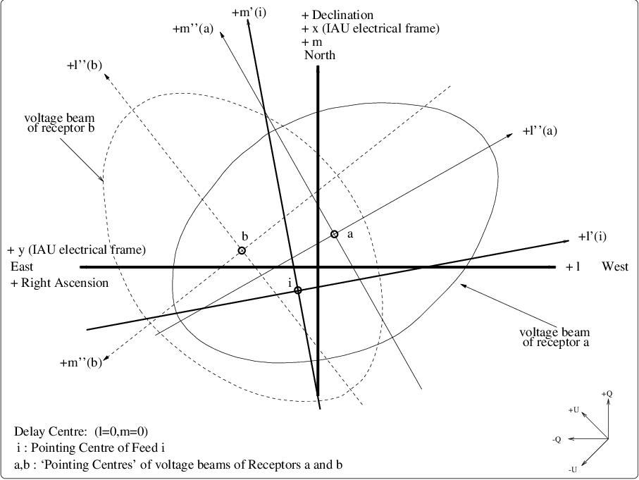
A.3 Coordinate frames
Fig 1 gives an overview of the coordinate system(s) used. All angles on the Sky are measured counter-clockwise,
i.e. in the direction North through East. When relevant, ‘axis’ means ‘positive axis’ (e.g. the positive
-axis).
It is important to make a distinction between:
The beam frame(s): In order to calculate the effects of the primary beam on the signal of a source in
direction ,
the shape and position of the voltage beams of each receptor on the Sky has to be calculated. For
fully steerable parabolic antennas, which have constant beamshapes, this can be done most
conveniently in coordinate frames defined by the projected position angles of the receptors. To allow
for the fact that the two beams of a feed are closely coupled, an intermediate feed-frame is defined
also.
The electrical frame: For the polarisation of the signal, the only relevant parameters are the projected angles w.r.t.
the ‘electrical’ axes
and
defined by the IAU.
NB: In order to see that two frames are needed, consider that Faraday rotation rotates the electric
vector, but not the beam on the sky.
| Frame of the entire telescope (single dish or array): |
| | \vvAntPos | Projected feed (receptor?) position vector |
| | \ccU,\ccV,\ccW | Projected baseline coordinates |
| | \vvUVW | Projected baseline vector |
| Electrical frame on the sky (IAU definition): |
| | \ccX,\ccY | IAU electrical frame on the sky. |
| | \ccZ | propagation direction of incident field. |
| | \aaXY | Angle from -axis to -axis () |
| | \ccXPol,\ccYPol | linear polarisation coordinates. |
| | \ccRPol,\ccLPol | circular polarisation coordinates. |
| Sky frame (w.r.t. fringe stopping centre): |
| | \ccL,\ccM,\ccN | Coordinates (direction cosines) |
| | \vvLMN | Source direction vector |
| | \vvFTC | Fringe Tracking Centre |
| | \vvMC | Map Centre |
| | \aaLM | Angle from -axis to -axis () |
| | \aaLX | Angle from -axis to -axis () |
| Coordinate frame of feed , projected on the sky: |
| | \ccLI,\ccMI | Coordinates |
| | \ccLIO,\ccMIO | Origin () of feed-frame. |
| | \aaLI | Angle from -axis to -axis |
| | \aaXI | Angle from -axis to -axis () |
| Coordinate frame of receptor of feed , projected on the sky: |
| | \ccLIA,\ccMIA | Coordinates |
| | \ccLIAO,\ccMIAO | Origin () of receptor-frame. |
| | \aaIA | Angle from -axis to -axis |
| | \aaXA | Angle from -axis to -axis () |
| Coordinate frame of receptor of feed , projected on the sky: |
| | \ccLIB,\ccMIB | Coordinates |
| | \ccLIBO,\ccMIBO | Origin () of receptor-frame. |
| | \aaIB | Angle from -axis to -axis |
| | \aaYB | Angle from -axis (!) to -axis () |
The coordinates
and of the frames
of receptors and
in equ 37 are related to the
celestial coordinate frame
in a two-step process. First we define an intermediate feed-frame
for
feed ,
projected on the Sky:
|
| (55) |
in which is the Pointing
Centre of feed , and
is a rotation over the
projected angle between
the positive -axis of the
Sky frame and the -axis
of the feed-frame.
The voltage beams themselves are best modelled in a receptor-frame (see equ 37), again projected on the Sky.
For receptor
we have:
|
| (56) |
The matrix represents a rotation
over the angle between the
positive -axis of the feed-frame
and the -axis of the relevant
receptor-frame. For receptor :
|
| (57) |
and
represent pointing
offsets of receptor
and
respectively. These can be used to model ‘beam-squint’ of feeds that are not axially symmetric.
A.4 Matrices and vectors
The following matrices and vectors play a role in the Measurement Equation:
| | \vvIQUV | Stokes vector of the source (I,Q,U,V). |
| | \vvCoh,\vvCohEl | Coherency vector, and one of its elements. |
| | \mmStokes | Stokes matrix, conversion between polarisation representations. |
| | \mmStokes\ssLin | Conversion to linear representation. |
| | \mmStokes\ssCir | Conversion to circular representation. |
| | \mmMueller | Mueller matrix: Stokes to Stokes through optical ‘element’ |
| | \mmXifr,\mmXifrEl | Correlator matrix (). |
| | \mmMifr,\mmMifrEl | Multiplicative interferometer-based gain matrix (). |
| | \vvAifr,\vvAifrEl | Additive interferometer-based gain vector. |
The following feed-based Jones matrices
have a well-defined meaning:
| | \mjJones,\mjJonesEl | Jones matrix, and one of its elements. |
| | \mjFrot,\mjFrotEl | Faraday rotation (of the plane of linear pol.) |
| | \mjTrop,\mjTropEl | Atmospheric gain (refraction, extinction). |
| | \mjProj,\mjProjEl | Projected receptor angle(s) w.r.t. frame |
| | \mjBtot,\mjBtotEl | Total feed voltage pattern (i.e. . |
| | \mjBeam,\mjBeamEl | Traditional feed voltage beam. |
| | \mjConf,\mjConfEl | Feed configuration matrix (...). |
| | \mjDrcp,\mjDrcpEl | Leakage between receptors and . |
| | \mjHybr,\mjHybrEl | Hybrid network, to convert to circular pol. |
| | \mjGrec,\mjGrecEl | feed-based electronic gain. |
| | \mjKern,\mjKernEl | Fourier Transform Kernel (baseline phase weight) |
| | \mjKref,\mjKrefEl | FT kernel for the fringe-stopping centre. |
| | \mjKoff,\mjKoffEl | FT kernel relative to the fringe-stopping centre. |
| | \mjQsum,\mjQsumEl | Electronic gain of tied-array feed after summing. |
| Some special matrices and vectors: |
| | \mjDiag | Diagonal matrix with elements |
| | \mjMult | Multiplication with factor |
| | \mjRot | [pseudo] Rotation over an angle , |
| | \mjEll | Ellipticity angle[s] , |
| | \mjLtoC | Signal conversion from linear to circular. |
| | \mjCtoL | Signal conversion from circular to linear. |
Definitions of some special matrices:
|
| (58) |
A ‘pure’ rotation is a special
case of a ‘pseudo rotation’ :
|
| (59) |
Ellipticity:
|
| (60) |
A.5 Miscellaneous parameters
| | \ppParall | Parallactic angle, form North pole to zenith |
| | \ppLAT | Latitude on Earth |
| | \ppFarad | Faraday rotation angle |
| | \ppRcpPosDev | Dipole position angle error |
| | \ppRcpEllDev | receptor ellipticity |